Designed more than century ago, Gantt chart is very popular to the Project Manager communities and decision makers. This is equally important to project team.
It is a horizontal bar chart that shows activities over time with additional details on the same chart. We will create a template for Gantt chart in google sheets together. You would also be able to download the template. If you are only interested in the template, please scroll down and download the template.
The Template we are going to create in google sheets will have all the following elements of modern gantt chart
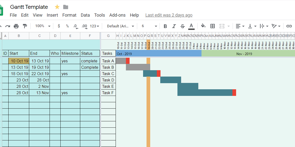
Gantt chart in our google sheet example
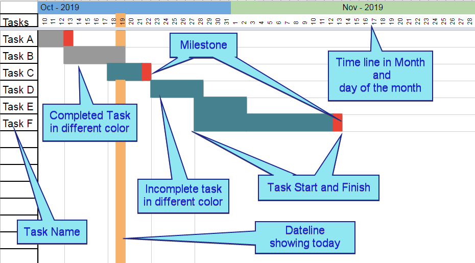
- List of Tasks
- Timeline in Month and day of the Month
- Task start and finish
- How long each task will take
- Who is working on each task
- Milestone
- Dateline
- The finish date of the project.
Let's see how our gantt chart is going to look like
How to build the gantt chart in google sheets using conditional formatting
We will simple conditional formatting to create our gantt chart.
Steps:
- Create Headers: Take a blank google sheets and put the data columns from second rows (A2): ID, Start Date, End Date, Who, Milestone, Status, Tasks. Here, Start Date and End Date is used to create the horizontal bar representing the Tasks. Milestone field is used to mark the end of task as milestone. Status is used to change the color of the bar as inactive
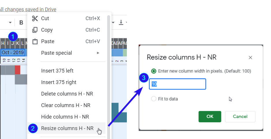
- Change Column width: Select column H till NM (H:NM). right click on the column heading and change column width to 10 pixels. Each of this column would be used to represent a day
- Populate dates for Timeline: We use Cell B3 to put the first task of the Project. the Gantt chart starts with that date. so on Cell H2 type in =B3. On I2 put H2+1 and copy I2 to all the cell through NM2
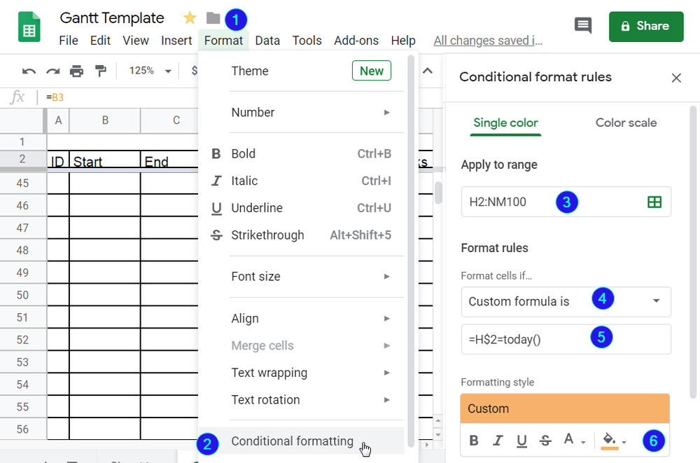
- Create dateline using Conditional Formatting: This the vertical line representing today. We will create for 100 rows. So, let's select H2:NM100. Click on Format Menu->Conditional Formatting. On the the new pop-up ensure that Apply ranges to shows H2:NH100. select Custom Formula is in the Format rules. Write =H$2=today() and then select the day colorin the formatting style. Please refer to the picture below
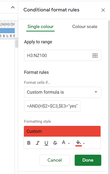
- Create Marker for Milestone (if E column have yes): The last part of preparing the template is representing the task on horizontal line according to the start and end date. Almost same as previous step. We select H3:NH100 instead of H2:NH100 and add Custom Formulas by choosing Custom formula is from drop down. Add the following =AND(H$2=$C3,$E3="yes") . Also, please remember to change the color from the Fill color drop down and choose your favorite color for Milestone
- Create Gantt Chart horizontal line using conditional formatting for completed Tasks:
- Please repeat the same task sequence as above. to create one more Conditional formatting. But this time the formula would be the following: =IF(OR(isblank($B3),isblank($C3)),False,AND(H$2>=$B3,H$2<=$C3,$F3="complete"))
- Color of the bar to be selected from Fill Color dropdown. we have used dark grey for completed tasks
- Create Gantt Chart horizontal line using conditional formatting for non-completed tasks:
- Please repeat the same task sequence as above. to create one more Conditional formatting. But this time the formula would be the following: =IF(OR(isblank($B3),isblank($C3)),False,AND(H$2>=$B3,H$2<=$C3))
- Color of the bar to be selected from Fill Color dropdown. we have used dark cyan for non-completed tasks
Now at the last part I will share the template that we have created together. You should check yourself to see how I have implemented Automatic Month and Year name and difference in the color. It is all in the conditional formatting. I think you will love finding that yourself
Here is the template Gantt Chart Template using conditional formatting . You can open it online and make a copy for yourself and use it.
You can reuse the template by replacing the data from your data table. Just ensure that
The Columns are matching. Like data of start date of tasks has to match start date of the template. Hope this will be useful