An obvious expectation from a decent Task tracker or Project tracker is to have a visual of tasks that needs attention. This could be the tasks or activities that are in progress or may be past due.
Here, we will build a template together, so that if any minor change is needed that can be don in the template. This is a simple tracker based on Conditional formatting. Will walk you through the simple steps. But if you are in hurry and interested in the template only, please feel free to download it here.
How it works
Excel has built-in features to show Icons representing status. This can be achieved through Conditional formatting. But there are some limitations. This is basically based on the value of the cell itself. So, the value based on which the icon is changing is not visible. Another issue is that the number of Icons in icon sets are maximum 4. If we need to handle more than four scenario, then the Conditional formatting will not work.
To overcome the situation, in this approach a dedicated column been created. This column will show the extended RAG (Red, Amber, Green) status based on some other columns.
Here, for each color, we will create Conditional Formatting. Let's assume that our Task tracker will have more or less 25 Tasks. So we will apply conditional formatting for fewer lines
The trick we will use here to change the Font color of a cell and then type in a symbol e.g. 🟠 that you would like to change color
Font color would be the background color of the excel sheet. So, if there is no color selected for the cells, then the font for the cell would be set to white manually. Conditional formatting will be changing font color of the tests in the cell
Let's type or insert a symbol (Insert toolbar menu -> Symbols ->Symbol ) or emoji (Win + Period ) in C2 and fill down for the cells that you populate
Status is Green:
If the "Status" field contains the word "Done", then make the RAG status Green
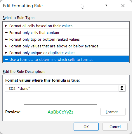
Let's select Status field column (C column ) upto row 25 and click on Conditional formatting and then New Rule. Then Use Formula... as shown in the picture below. Next, we need to change the font color to green. This can be done by clicking on Format and choosing Color Green in the Font Tab
=$D2="done"
RAG is Blue:
We will repeat the process that we have used for the "Status in Green" Steps. But the formula would be different and the font color would be Blue.
=AND(D2<>"done",F2>TODAY()+5)
Here, we are making sure that the Task not in "Done" state and that the task due date is more than 5 days in the future. If your requirement is different, for example you want to color it based on the start date, please change the formula accordingly. It is important that the Conditional formattings are added in the same sequence. Otherwise, some conditions it might behave differently
Past Due in Red:
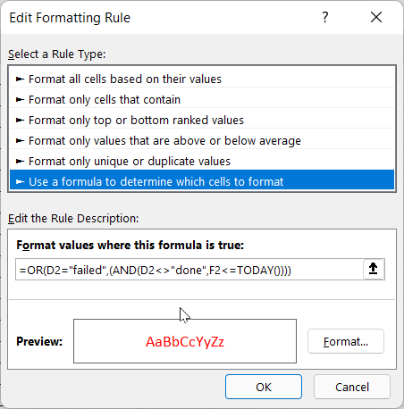
We will repeat the process that we have used for the "Status in Green" Steps. But the formula would be different and the font color would be Red.
=OR(D2="failed",(AND(D2<>"done",F2<=TODAY())))
and finally, it will look like the pic below
RAG status Amber:
Again, we will repeat the process that we have used for the "Status in Green" Steps. But the formula would be different and the font color would be Amber. Condition that I made here is that the Task is not in "Done" state and that the due date is within next 5 days
Finally, it would look like the picture above. If you are looking for the template and it is just sufficient, here you go ... grab the excel template